Fire Mapping with ArcGIS
This tutorial replicates part of the Los Angeles Fire Department (LAFD) Air Operations (Air Ops) data processing workflow. It demonstrates how to use rapidly calculated longitude and latitude values for flight path points, convert selected points into a closed polygon, and calculate perimeter and area for a selected flight polygon using ArcGIS 9.1 and a third-party ArcGIS extension, XTools Pro.
What Is GIS?
Making decisions based on geography is basic to human thinking. Where shall we go, what will it be like, and what shall we do when we get there are applied to the simple event of going to the store or to the major event of launching a bathysphere into the ocean's depths. By understanding geography and people's relationship to location, we can make informed decisions about the way we live on our planet. A geographic information system (GIS) is a technological tool for comprehending geography and making intelligent decisions.
GIS organizes geographic data so that a person reading a map can select data necessary for a specific project or task. A thematic map has a table of contents that allows the reader to add layers of information to a basemap of real-world locations. For example, a social analyst might use the basemap of Eugene, Oregon, and select datasets from the U.S. Census Bureau to add data layers to a map that shows residents' education levels, ages, and employment status. With an ability to combine a variety of datasets in an infinite number of ways, GIS is a useful tool for nearly every field of knowledge from archaeology to zoology.
A good GIS program is able to process geographic data from a variety of sources and integrate it into a map project. Many countries have an abundance of geographic data for analysis, and governments often make GIS datasets publicly available. Map file databases often come included with GIS packages; others can be obtained from both commercial vendors and government agencies. Some data is gathered in the field by global positioning units that attach a location coordinate (latitude and longitude) to a feature such as a pump station.
GIS maps are interactive. On the computer screen, map users can scan a GIS map in any direction, zoom in or out, and change the nature of the information contained in the map. They can choose whether to see the roads, how many roads to see, and how roads should be depicted. Then they can select what other items they wish to view alongside these roads such as storm drains, gas lines, rare plants, or hospitals. Some GIS programs are designed to perform sophisticated calculations for tracking storms or predicting erosion patterns. GIS applications can be embedded into common activities such as verifying an address.
From routinely performing work-related tasks to scientifically exploring the complexities of our world, GIS gives people the geographic advantage to become more productive, more aware, and more responsive citizens of planet Earth.
Modeling GPS Data Captured on the Fly
By Mike Price and Amy Fox, Entrada/San Juan, Inc.
This tutorial replicates part of the Los Angeles Fire Department (LAFD) Air Operations (Air Ops) data processing workflow. It demonstrates how to use rapidly calculated longitude and latitude values for flight path points, convert selected points into a closed polygon, and calculate perimeter and area for a selected flight polygon using ArcGIS 9.1 and a third-party ArcGIS extension, XTools Pro. For background information on the development of this workflow, see the accompanying article, "Tragedy to Triumph."

This tutorial creates the point flight path and derives an incident polygon from data collected during a training flight by LAFD Air Ops.
Getting Started
What You Will Need
- ArcGIS 9.x (ArcView, ArcEditor, or ArcInfo license level)
- Evaluation copy of XTools Pro downloaded from www.xtoolspro.com/download
- Sample dataset from ArcUser Online
- WinZip or other similar zipping utility
Visit ArcUser Online (www.esri.com/arcuser) and download the zipped archive containing the data for this exercise. Unzip the archive and open ArcCatalog to view the files. The archive creates a parent directory named FireMap that contains two sub directories, one for shapefiles and one for grid files. The grid files are registered in California State Plane North American Datum of 1983 (NAD83) Zone V U.S. Feet. Most shapefiles are registered in California State Plane with the exception of the training data file TR1_060316_1122 that was created in the World Geodetic System 1984 (WGS84) geographic coordinate system.
Next, visit Data East's download portal at www.xtoolspro.com/download and obtain a 30-day evaluation copy of the XTools Pro extension. Table 1 summarizes XTools Pro features and functions. Many basic functions are available in the free download while additional functionality can be purchased online. This tutorial uses these three free functions:
- Add XYZ Coordinates
- Make One Polygon from Points
- Calculate Area, Perimeter, Length, Acres and Hectares
After downloading and extracting the XTools Pro archive, navigate to the directory containing the XTools Pro 3.2.0 folder and double-click the setup.exe file. After working through the setup wizard, verify the program has been installed by navigating to \ProgramFiles\DataEast\XToolsPro3. Restart ArcMap. Enable the XTools Pro extension by choosing Tools > Extensions from the Standard menu and checking the box next to the XTools Pro extension. Close the Extensions dialog box. In the Standard menu, choose View > Toolbars and add the XTools Pro toolbar.
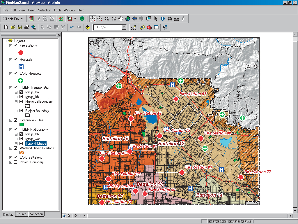
Add the shapefiles and hillshade to create a basemap for the training data.
Building a Basemap
- Start ArcMap and open a new map document.
- Navigate to FireMap\SHPFiles\CASP835F\ and add the Project Boundary LYR file to the Data Frame. If the data connection in the layer file is broken, right-click Project Boundary's name in the table of contents (TOC), choose Data > Set Data Source, and navigate to FireMap\SHPFiles\CASP835F\Clippol1.
- Open the Data Frame properties and verify that the Project Boundary data has set the coordinate system to CA State Plane NAD83 Zone V US Feet. Click the General tab and rename the Data Frame CA State Plane NAD83 Zone V US Feet.
- Load the remaining layer files stored in the FireMap\SHPFiles\CASP835F folder. Each LYR file should load the appropriate shapefile or grid and associate it with the desired thematic legends. Repair any broken links by right-clicking on the layer file in the TOC, selecting Data > Set Data Source, navigating to FireMap\SHPFiles\CASP835F\, and selecting the shapefile corresponding to the layer file.
- Add the Topo Hillshade layer stored in FireMap\GRDFiles\CASP835F and arrange the TOC data layers in the following order (top to bottom):
Fire Stations
Hospitals
LAFD Helispots
TIGER Transportation
Municipal Boundary
Project Boundary
Evacuation Sites
TIGER Hydrography
Topo Hillshade (transparency set to 50 percent)
Wildland Urban Interface (no forward slash between Wildland and Urban!)
LAFD Battalions (labeled)
- Save the map in the FireMap folder and name it FireMap1. Become familiar with the data layers and check out the attributes for each.
Loading Flight Path Data
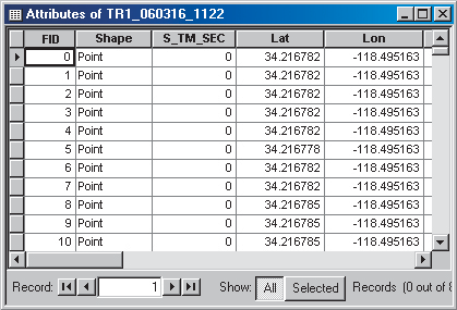
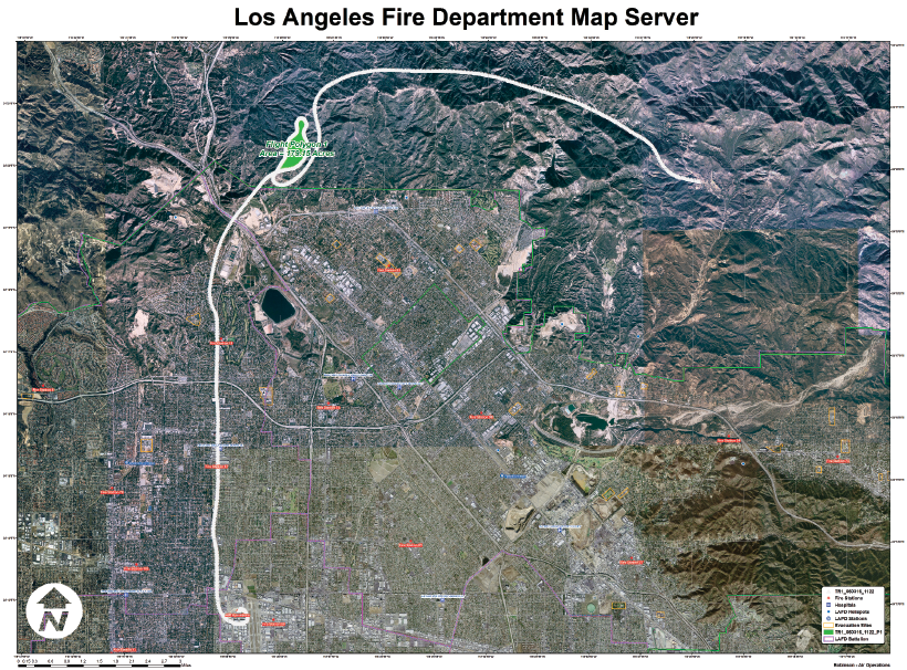
With the basemap created, the GPS data can be added to the map document. This data was gathered during a training flight in northern Los Angeles County on March 16, 2006. Navigate to FireMap\SHPFiles\LatLon84 and load TR1_060316_1122, a single point shapefile. Its name, TR1_060316_1122, indicates that it was collected during a training flight by Airship 1 on March 16, beginning at 1122 (i.e., 11:22 a.m. Pacific standard time). An ArcMap dialog box will warn that the data was created in another projection and will be transformed to California State Plane. Inspect this data and its attribute table. The flight began at Air Ops headquarters at the Van Nuys Airport, then traveled east over the San Gabriel foothills.
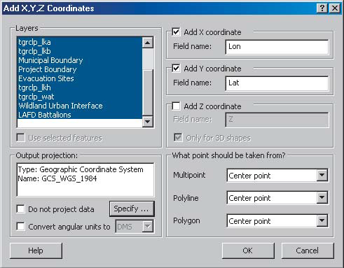
Calculating Longitude and Latitude Values for Flight Points
XTools Pro will be used to calculate the X- and Y-coordinates for the flight paths. In the TOC, right-click the TR1_060316_1122 point layer and choose Open Attribute Table. Notice that the Lat and Lon fields contain zero values. These fields will be updated with coordinates in decimal degrees WGS84.
|
 |
Measuring Flight Paths and Calculating Ground Speed
Zoom into the map just north of where the flight path crosses above Fire Station 87 so that the map scale is 1:5,000. Select 17 points north of the station that represent one-half mile of flight line. Looking at this data, how fast was the helicopter flying? (Hint: Measure the distance between point 0 and point 16. Each point represents one second of air time. Traveling one-half mile in 16 seconds represents a ground speed of 112.5 mph, or slightly less than two miles per minute.)
Retracing the Flight Path
Reset the map scale to 1:12,000 and pan north along the flight points to the loop in the flight path (i.e., where the flight path crosses itself). It traces the perimeter of an area of interest. The UltiChart
navigation unit in the helicopter accurately captured this boundary. Using the Select Features tool, capture the two points just outside the closed loop. Open the Attribute Table and click Show: Selected Records to display only those features (FID points 344 and 476). Confirm that the airship required just over two minutes to fly this perimeter. Did you notice that the helicopter was flying in a counterclockwise direction? Because the pilot sits in the right seat, this perimeter path was guided by the navigator in the left seat.
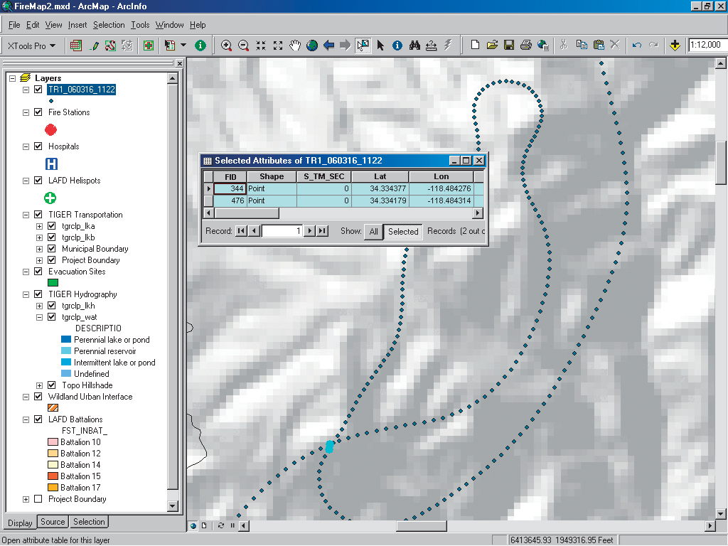
The flight loop shows an area of interest. Using the Select Features tool, capture the two points just outside of the closed loop. Open the attribute table and click on Show: Selected Records to display only those features (FID points 344 and 476).
Creating a Closed Polygon from Points with XTools Pro
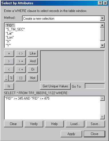
Boolean logic can be used to define the polygon area of the flight path by selecting the points that initialize the loop and writing a query to limit the shape of the flight path to these points. Can you determine where the loop originates and ends? Note the lowest and highest FID numbers of the two points inside the loop are 345 and 475.
|
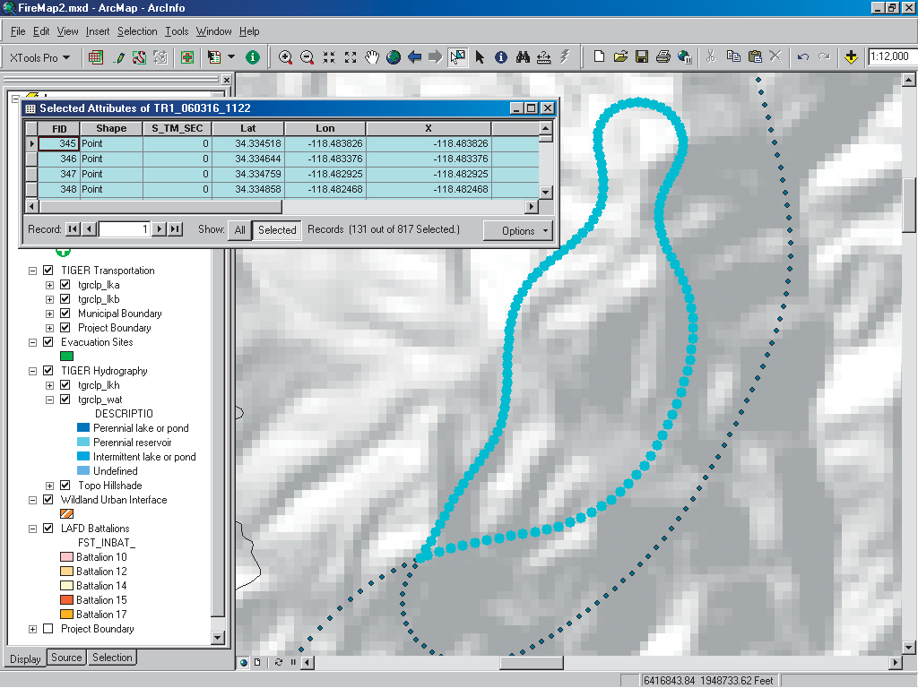
Choose the Select by Attributes dialog box, and use a query to select all the points in the loop. |
Calculating Perimeter and Area
- Right-click TR1_060316_1122_P1 and choose Zoom to Layer. Open this layer's attribute table. Move the table in the lower left part of the display.
- Click the XTools Pro drop-down arrow on the XTools toolbar. Choose Select Table Operations >Calculate Area, Perimeter, Length, Acres and Hectares. In the Calculate window, locate Output Projection and click Specify.
Click the XTools Pro drop-down arrow on the XTools toolbar and choose Select Table Operations > Calculate Area, Perimeter, Length, Acres and Hectares.
- Click the Specify button in the Spatial Reference Properties dialog box and choose Projected Coordinate Systems. Navigate to State Plane, then NAD 83 (Feet), and select NAD 83 StatePlane California V FIPS 0405 (Feet).prj. Click Add, OK, and OK. Change desired output units to Feet. This is a critical and easy to miss step! Accept all other default selections and click OK. The attributes now include measurements. Minimize the Attribute Table and save the project.
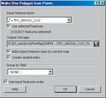 A polygon can be created from this poly point selection.
|
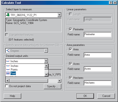 When using the Calculate Area, Perimeter, Length, Acres and Hectares function in XTools Pro, be sure to change the input units to feet.
|
Validating and Labeling the Polygon
- Use the Identify tool to verify that the new polygon has an area of 179.147730 acres. To create a label, right-click TR1_060316_1122_P1 and select Properties. Choose the Labels tab and click the Expressions button. In the Expressions box, type: "Flight Polygon" & [ID]+1&VBNewLine & ROUND([Acres],2) & " Acres" Be certain to insert a leading space before the text " Acres". Click Verify to confirm the expression and label format. Click OK twice to exit both dialog boxes.
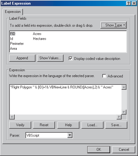
Use an expression to label the new polygon.
- In the Layer Properties dialog box, click Symbol. In the Symbol Selector dialog box, click Properties. Click the Mask tab and set the Halo to 2.00 points. Click OK. In the Symbol Selector dialog box, choose Arial font at 18 points, bold, italic. Click OK.
- In the Layer Properties dialog box, check Label features in this layer. Click OK and apply the new label properties to the map. Verify that the label was successfully created.
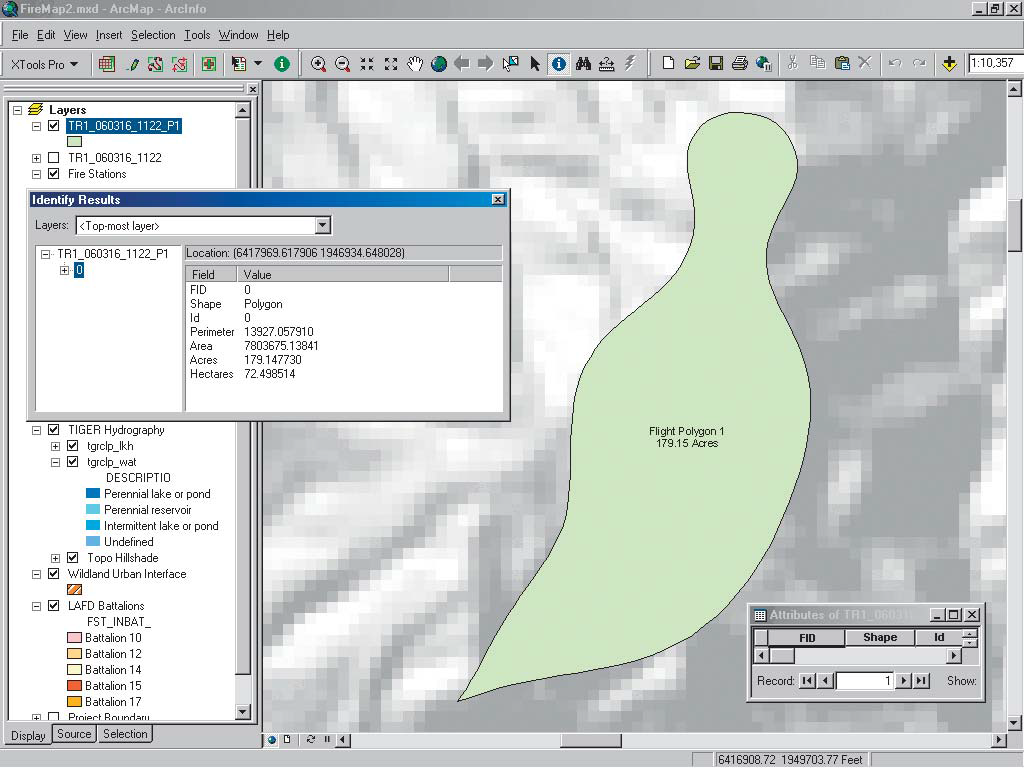
The finished flight polygon is labeled with the area of the polygon.
Summary
This tutorial creates the point flight path and derives an incident polygon from data collected during a training flight by LAFD Air Ops. LAFD's mapping program is growing rapidly. Steven Robinson, the program's creator, envisions the day when a captured polygon, merged with current demographic information, will be transferred to incident managers in real time. When processed by reverse 911, citizens at risk may be quickly alerted. Through careful program design, staff training, current data development, and support from LAFD management and technology providers, Robinson's dream is within reach.
This tutorial replicates part of the Los Angeles Fire Department (LAFD) Air Operations (Air Ops) data processing workflow. Rapidly calculated longitude and latitude values for flight path points are converted into a closed polygon and the perimeter and area calculated.
Tragedy to Triumph
Pilot's Vision Leads to Onboard State-of-the-Art Mapping
 |
In March 1998, three Los Angeles city firefighters and a young girl being transported to a hospital were killed in a helicopter crash in the Griffith Park area of Los Angeles, California. Steven Robinson, the helicopter's pilot, was one of two crew members who survived the crash. Despite several years of rehabilitation, Robinson was unable to return to active flight status. However, instead of leaving the Air Operations (Air Ops) service, Robinson developed and implemented a state-of-the-art data capture, analysis, and mapping program that provides the Los Angeles Fire Department (LAFD) airships with high-quality current maps on-board and a current common operating picture (COP) to emergency managers and responders for a wide range of emergency and non-emergency events. When Robinson discovered that the GPS-based on-board navigation system for the department's helicopter fleet accurately captured an airship's position during every second of flight, he envisioned a process for carefully tracing and recording the perimeter of emergencies and other events such as wildland fires, hazmat accidents, natural disasters, and public gatherings. |
In 2002, Robinson approached ESRI to request assistance with mapping technology, data development, and real-time mapping. Russ Johnson, ESRI's public safety solutions manager, recognized the value of Robinson's idea. With technical assistance from ESRI and hardware donated by Hewlett-Packard, Robinson's helicopter mapping program literally took off. As the program has grown, it has been recognized by the City of Los Angeles, neighboring communities, and adjoining counties. Robinson received many more requests for mapping services than he could handle. He decided to develop and support a standard data capture workflow, template-based incident mapping, and a training program that would empower helicopter pilots, flight medics, and firefighters to participate in aerial data collection and emergency mapping.
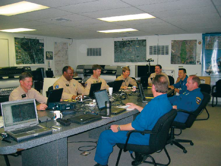
In early 2006, ESRI sponsored a program to define a standard workflow and train Air Ops mapping staff. Project requirements included capturing high-quality GPS points and rapidly transferring these points to a modeling computer. First, the GPS points are managed and filtered to map flight paths and incident boundaries. Next, the points are converted to polygons and perimeters and those areas are calculated. The map elements are then posted in a standard map template for plotting and delivery to incident managers.
Acknowledgments
The authors thank Los Angeles Fire Department pilot Steven Robinson, Air Operations Battalion Chief John Buck, and the entire helicopter crew for their support and interest. Special thanks are also extended to ESRI, IBM/Lenovo, and HP for providing software, hardware, and program technical support.
(Reprinted from the July–September 2006 issue of ArcUser magazine)